
Estimating cable life is inherently uncertain and should normally be treated as an engineering estimate rather than a precise prediction. A key factor is the temperature at which the cable insulation operates over time.
IEC 60216 provides guidance on estimating the thermal endurance of insulating materials from measurements on test samples. For a particular cable construction, manufacturer data should be used where it is available.
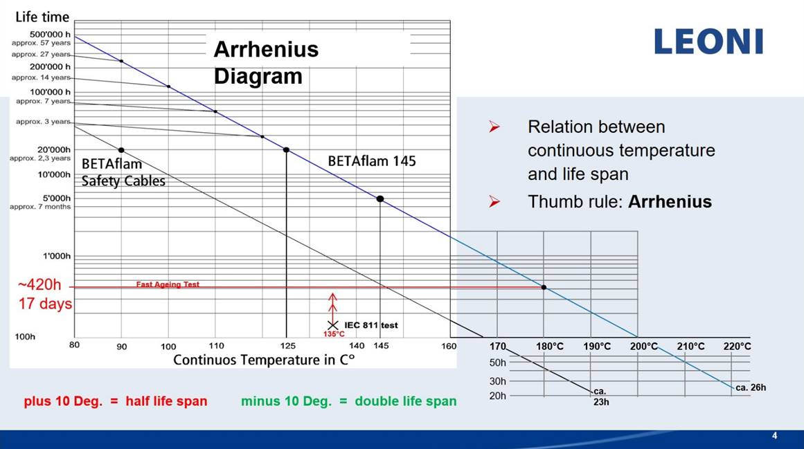
This topic sits alongside Cable Insulation and Cable Thermal Analysis: the insulation material sets the thermal limit, while the installation determines the operating temperature.
Arrhenius equation
An Arrhenius-type relationship is often used to estimate insulation ageing and life expectancy as a function of temperature:
| k | Expected life, h |
| A | Pre-exponential factor |
| E | Activation energy |
| R | Boltzmann or gas constant, depending on units used for E |
| T | Temperature, K |
Taking the natural logarithm and rearranging gives a straight-line relationship:
Because A, E and R are constants for a fitted material model, the result can be plotted as a straight line. In practice, engineers normally fit the relationship to manufacturer test data rather than relying on generic constants.
Rule of thumb
A common rule of thumb is that every 10 °C rise in operating temperature halves insulation life. Conversely, a 10 °C reduction in operating temperature doubles insulation life. This rule is a simplified consequence of Arrhenius-type ageing behaviour and should be used with care.
Application example
From manufacturer data, the temperature-life relationship may be treated as log-linear:
Using the example values shown in the source data, the slope is:
The intercept is:
Therefore:
At 110 °C, the estimated life is:
The result is only as good as the ageing model and the underlying test data. Real cable life also depends on installation conditions, load profile, moisture, mechanical damage, voltage stress, accessories and manufacturing details.